注意：基于参考原因，本文参杂了APM的算法分析。

本篇文章首先简述了下px4和apm调用姿态相关应用程序出处，然后对APM的DCM姿态解算算法参考的英文文档进行了翻译与概括，并结合源代码予以分析，在此之前，分析了starlino的DCM，并进行了matlab的实现，因为它更加利于理解。后段时间会对px4的四元数姿态解算进行分析。姿态控制部分描述了串级PID在APM里的实现流程，同样后期会完善对px4的分析。最后针对自己平时使用的一些调试技巧进行了总结。

姿态出处分析

下面看下重要的一个脚本/etc/init.d/rc.mc_apps，可以知道姿态估计用的是attitude_estimator_q和position_estimator_inav，用户也可以选择local_position_estimator、ekf2，而姿态控制应用为mc_att_control和mc_pos_control。

1
2
3
4
5
6
7
8
9
10
11
12
13
14
15
16
17
18
19
20
21
22
23
24
25
26
27
28
29
#!nsh
if param compare INAV_ENABLED 1
then
	attitude_estimator_q start
	position_estimator_inav start
else
	if param compare LPE_ENABLED 1
	then
		attitude_estimator_q start
		local_position_estimator start
	else
		ekf2 start
	fi
fi

if mc_att_control start
then
else
	# try the multiplatform version
	mc_att_control_m start
fi

if mc_pos_control start
then
else
	# try the multiplatform version
	mc_pos_control_m start
fi
...

而在ardupilot中，姿态解算与控制算法在ArduCopter.cpp的fast_loop任务中以400Hz的频率运行。

// Main loop - 400hz
void Copter::fast_loop()
{

    // IMU DCM Algorithm
    // --------------------
    read_AHRS();
    ...
}

void Copter::read_AHRS(void)
{
	...

    ahrs.update();
}

了解了上面的源码出处后，下面将分具体应用进行分析。

姿态传感器数据采集

首先进行传感器的初始化，主要步骤为：关闭软件低频滤波器、设置传感器量程、关闭硬件低频滤波器、设置采样频率、设置队列深度，具体实现如下：

// software LPF off
ioctl(fd, ACCELIOCSLOWPASS, 0);
// 16g range
ioctl(fd, ACCELIOCSRANGE, 16);
switch(devid) {
    case DRV_ACC_DEVTYPE_MPU6000:
    case DRV_ACC_DEVTYPE_MPU9250:
        // hardware LPF off
        ioctl(fd, ACCELIOCSHWLOWPASS, 256);
        // khz sampling
        ioctl(fd, ACCELIOCSSAMPLERATE, 1000);
        // 10ms queue depth
        ioctl(fd, SENSORIOCSQUEUEDEPTH, _queue_depth(1000));
        break;
    case DRV_ACC_DEVTYPE_LSM303D:
        // hardware LPF to ~1/10th sample rate for antialiasing
        ioctl(fd, ACCELIOCSHWLOWPASS, 194);
        // ~khz sampling
        ioctl(fd, ACCELIOCSSAMPLERATE, 1600);
        ioctl(fd,SENSORIOCSPOLLRATE, 1600);
        // 10ms queue depth
        ioctl(fd, SENSORIOCSQUEUEDEPTH, _queue_depth(1600));
        break;
    default:
        break;
}

然后以400HZ频率的循环任务通过SPI通信来采集传感器数据，并将采集到的数据进行纠错处理，如减去静态偏差量。此时，将采集到的这些数据同步写入SD卡，以便于飞行测试后期进行数据分析。这个过程的数据是以结构体的形式存放于全局变量imu中，后面进行姿态解算时直接读取该变量的值即可。同步写入SD卡实现如下：

DataFlash_Class *dataflash = get_dataflash();
if (dataflash != NULL) {
    uint64_t now = AP_HAL::micros64();
    struct log_GYRO pkt = {
       LOG_PACKET_HEADER_INIT((uint8_t)(LOG_GYR1_MSG+instance)),
        time_us   : now,
        sample_us : sample_us?sample_us:now,
        GyrX      : gyro.x,
        GyrY      : gyro.y,
        GyrZ      : gyro.z
    };
    dataflash->WriteBlock(&pkt, sizeof(pkt));
}

姿态估算

DCM_tutorial

imu_guide/imu_guide中文翻译/dcm_tutorial/wiki资料查询/该部分算法源码参考
将该算法转换为了matlab实现，想了解的可以查看我的github里的DCM工程，能够更好的理解算法，另外，该matlab实现还有一定的bug，希望各位大神的pull request~
这部分翻译自dcm_tutorial，并结合源码进行分析，可作为下部分DCM理论介绍的基础哦，所以建议先将这部分看完再往下看～

DCM矩阵：

设机体坐标系为Oxyz，与机体坐标系同x,y,z方向的单位向量为i, j, k。地理坐标系为OXYZ，同理地理坐标系的单位向量为 I, J, K。共同原点为O。如图

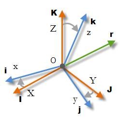
I$^G$ = {1,0,0}$^T$, J$^G$={0,1,0}$^T$ , K$^G$ = {0,0,1}$^T$
i$^B$ = {1,0,0}$^T$, j$^B$={0,1,0}$^T$ , k$^B$ = {0,0,1}$^T$
下面将i，j，k向量用地理坐标系表示，首先以i作为一个例子。
i$^G$ = {i$_x$$^G$ , i$_y$$^G$ , i$_z$$^G$}$^T$
其中i$_x$$^G$表示的是i向量在地理坐标系X轴上的投影，即
i$_x$$^G$ = |i| cos(X,i) = cos(I,i)
在这个式子中，|i|是i单位向量的范式（长度），cos(I,i)是向量I和向量i夹角的余弦，因此可以这样写：
i$_x$$^G$ = cos(I,i) = |I||i| cos(I,i) = I.i
在这个式子中，I.i是向量I和向量i的点积，由于只是计算点积，我们并不关心向量是在哪个坐标系中测量的，只要都是以同一个坐标系表示即可。所以：
I.i = I$^B$.i$^B$ = I$^G$.i$^G$ = cos(I$^B$.i$^B$) = cos(I$^G$.i$^G$)
同样的：
i$_y$$^G$ = J.i , i$_z$$^G$=K.i
所以i向量可以用地理坐标系表示为：
i$^G$= { I.i, J.i, K.i}$^T$
同样的，j，k向量可以表示为：
j$^G$= { I.j, J.j, K.j}$^T$ , k$^G$= { I.k, J.k, K.k}$^T$
将机体坐标i，j，k的地理坐标表示以矩阵的形式表示为：

这就是方向余弦矩阵，它是由机体坐标系和地理坐标系向量所有两两向量组合的夹角的余弦组成，可以算出共有9$\times$9种。
下一节的DCM理论里面有另外一种推理DCM的方法，建议交互思考！
而将地理坐标系在机体坐标系中表示与将机体坐标系在地理坐标系中表示是对称的，所以只需简单交换I, J, K 和 i, j, k即可。
I$^B$= { I.i, I.j, I.k}$^T$ , J$^B$= { J.i, J.j, J.k}$^T$ , K$^B$= { K.i, K.j, K.k}$^T$
转化为矩阵形式为：

很容易可以发现：
DCM$^B$ = (DCM$^G$)$^T$ or DCM$^G$ = (DCM$^B$)$^T$，换句话说，这两个矩阵是可以相互转换的。
也可以发现：
DCM$^B$. DCM$^G$ = (DCM$^G$)$^T$ .DCM$^G$ = DCM$^B$. (DCM$^B$)$^T$ = I$_3$
其中I$_3$为3$\times$3的单位矩阵，换句话说，DCM矩阵是正交矩阵。
证明如下：

证明这个我们需要知道这些特性：i$^{GT}$. i$^G$ = | i$^G$|| i$^G$|cos(0) = 1， i$^{GT}$. j$^G$ = 0，因为i和j是正交的。
方向余弦矩阵也称为旋转矩阵，如果知道机体坐标，则可以算出任意向量的地理坐标（反之同理），下面以机体坐标系向量使用DCM算出地理坐标作为例子进行推理：
r$^B$= { r$_x$$^B$, r$_y$$^B$, r$_z$$^B$}$^T$
而r$^G$ = { r$_x$$^G$ , r$_y$$^G$ , r$_z$$^G$ }$^T$
现在让我们分析第一个坐标r$_x$$^G$：
r$_x$$^G$ = | r$^G$| cos(I$^G$,r$^G$)，由于坐标系旋转，向量的大小，夹角都不会变，故有：
| r$^G$| = | r$^B$| , | I$^G$| = | I$^B$| = 1 ， cos(I$^G$,r$^G$) = cos(I$^B$,r$^B$)，所以：
r$_x$$^G$ = | r$^G$| cos(I$^G$,r$^G$) = | I$^B$ || r$^B$| cos(I$^B$,r$^B$) = I$^B$. r$^B$ = I$^B$. { r$_x$$^B$, r$_y$$^B$, r$_z$$^B$}$^T$
由上可知，r$^B$= { r$_x$$^B$, r$_y$$^B$, r$_z$$^B$}$^T$，替换得：
r$_x$$^G$ = I$^B$. r$^B$ = { I.i, I.j, I.k}$^T$ . { r$_x$$^B$, r$_y$$^B$, r$_z$$^B$}$^T$ = r$_x$$^B$ I.i + r$_y$$^B$ I.j + r$_z$$^B$ I.k
同样的思路：
r$_y$$^G$ = rx$^B$ J.i + ry$^B$ J.j + rz$^B$ J.k
rz$^G$ = rx$^B$ K.i + ry$^B$ K.j + rz$^B$ K.k
转化为矩阵形式为：

得证。
同样的思路可以证明：

也可以这样证明：
DCM$^B$ r$^G$ = DCM$^B$ DCM$^G$ r$^B$ = DCM$^{GT}$ DCM$^G$ r$^B$ = I$_3$ r$^B$ = r$^B$

角速度：

如下图所示，r为任意的旋转向量，t时刻的坐标为r(t)。时间间隔dt后：r = r (t) , r’= r (t+dt) and dr = r’ – r。

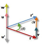
dt时间后向量r绕着与单位向量u同向的轴旋转了d$\theta$，停到了向量r’的位置。其中u垂直与旋转的机身，因此u正交于r与r’，图中显示了u与u’，它们与r和r‘的叉乘结果方向相同。故有
u = (r x r’) / |r x r’| = (r x r’) / (|r|| r’|sin(dθ)) = (r x r’) / (|r|$^2$ sin(dθ))
由于旋转并不改变向量的长度，因此有| r’| = |r|。
向量r的线速度可以表示如下：
v = dr / dt = ( r’ – r) / dt
当dθ → 0时，向量r和dr的夹角$\alpha$可通过r，r’和dr组成的等腰三角形计算：
α = (π – dθ) / 2 当dθ→ 0时，α → π/2。
这告诉我们，当dt → 0时，r垂直于dr，因此r ⊥ v （v和dr的方向是一致的）。
现在定义角速度向量，其中反应了角度的变化率和旋转轴方向。
w = (dθ/dt ) u
下面分析w和v之间的关系：
w = (dθ/dt ) u = (dθ/dt ) (r x r’) / (|r|$^2$ sin(dθ))
当dt → 0时，dθ → 0，因此sin(dθ) ≈ dθ。化简得：
w = (r x r’) / (|r|$^2$ dt)
现在由于 r’ = r + dr , dr/dt = v , r x r = 0，利用叉乘的加法分配率可得：
w = (r x (r + dr)) / (|r|$^2$ dt) = (r x r + r x dr)) / (|r|$^2$ dt) = r x (dr/dt) / |r|$^2$
最后得出：
w = r x v / |r|$^2$
下面反向推理证明v = w x r
利用向量的三重积公式：(a x b) x c = (a.c)b – (b.c)a，以及v和r是垂直的，所以v.r = 0
w x r = (r x v / |r|$^2$) x r = (r x v) x r / |r|$^2$ = ((r.r) v + (v.r)r) / |r|$^2$ = ( |r|$^2$ v + 0) |r|$^2$ = v
得证。

陀螺仪及角速度向量

如果我们定期获取陀螺仪的值，时间间隔为dt，那么陀螺仪将会告诉我们在这段时间，地球绕陀螺仪各轴旋转的度数。
dθ$_x$ = w$_x$dt，dθ$_y$ = w$_y$dt，dθ$_z$ = w$_z$dt
其中w$_x$ = w$_x$ i = {w$_x$ , 0 , 0 }$^T$ , w$_y$ = w$_y$ j = { 0 , w$_y$ , 0 }$^T$ , w$_z$ = w$_z$ k = { 0 , 0, w$_z$ }$^T$
每次旋转都会产生线性的位移
dr$_1$ = dt v$_1$ = dt (w$_x$ x r) ; dr$_2$ = dt v$_2$ = dt (w$_y$ x r) ; dr$_3$ = dt v$_3$ = dt (w$_z$ x r) .
矢量相加：
dr = dr$_1$ + dr$_2$ + dr$_3$ = dt (w$_x$ x r + w$_y$ x r + w$_z$ x r) = dt (w$_x$ + w$_y$ + w$_z$) x r
因此线速度可以表示为：
v = dr/dt = (w$_x$ + w$_y$ + w$_z$) x r = w x r
这里的条件是dt很小才能这么推理，也就是说，dt越大误差也就越大。

基于6DOF或者9DOF的IMU传感器DCM互补滤波算法

科普：6DOF由三轴陀螺仪和三轴加速度计组成，9DOF由三轴磁力计、三轴陀螺仪和三轴加速度计组成。
定义右手地理坐标系：I指向北方，K指向顶部，J指向西方。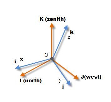

IMU组成机体坐标系，IMU包括陀螺仪、加速度计等。
加速度计能感应重力，重力向量指向地心，与顶部向量K$^B$方向相反，假如加速度计输出为A = {A$_x$ , A$_y$ , A$_z$ }，则K$^B$ = –A。
磁力计与加速度计相似，除了磁力计可以感应地理的北方以外，假设正确的磁力计输出为M = {M$_x$ , M$_y$ , M$_z$ }，由于I$^B$是指向北方，因此I$^B$ = M.
现在可以计算出J$^B$ = K$^B$ x I$^B$。
所以加速度计和磁力计就能单独的给出DCM矩阵：
DCM$^G$ = DCM$^{BT}$ = [I$^B$, J$^B$, K$^B$]$^T$
DCM矩阵能转换机体坐标系中的任意向量到地理坐标系中：
r$^G$ = DCM$^G$ r$^B$

加速度计和磁力计都需要初始化校正和纠错。
陀螺仪没有绝对的方向感，比如它不知道北方和顶部在哪里，但加速度计和磁力计知道，因此当我们知道t时刻的方向，矩阵形式表示为DCM(t)，那么我们可以用陀螺仪算出更精确的方向DCM(t+1)，所以这就是从带有噪音的加速度计或者有磁场干扰的磁力计估算出来的姿态。
事实是我们可以利用陀螺仪、加速度计和磁力计融合来估算姿态。下面将介绍这种算法：
地理坐标系表示的DCM矩阵如下：

该DCM矩阵的各行为I$^B$, J$^B$, K$^B$向量。我们会将重心放在K$^B$（由加速度计测定），I$^B$（由磁力计测定）上。 J$^B$可以由J$^B$ = K$^B$ x I$^B$计算出来。
假设机体坐标的顶部向量在t$_0$时刻表示为K$^B$$_0$，陀螺仪的输出为 w = {w$_x$ , w$_y$ , w$_z$ }，一段时间后，该顶部向量表示为K$^B$$_1G$
K$^B$$_1G$ ≈ K$^B$$_0$ + dt v = K$^B$$_0$ + dt (w$_g$ x K$^B$$_0$) = K$^B$$_0$ + ( dθ$_g$ x K$^B$$_0$)
其中dθ$_g$ = w$_g$dt为三个轴角度的变化向量，这意味这在dt时间内K$^B$向量在3个轴改变的角度。w$_g$为陀螺仪测得的角速度。
程序如下：

//---------------
//dcmEst
//---------------
//gyro rate direction is usually specified (in datasheets) as the device's(body's) rotation 
//about a fixed earth's (global) frame, if we look from the perspective of device then
//the global vectors (I,K,J) rotation direction will be the inverse
float w[3];					//gyro rates (angular velocity of a global vector in local coordinates)
w[0] = -getGyroOutput(1);	//rotation rate about accelerometer's X axis (GY output) in rad/ms
w[1] = -getGyroOutput(0);	//rotation rate about accelerometer's Y axis (GX output) in rad/ms
w[2] = -getGyroOutput(2);	//rotation rate about accelerometer's Z axis (GZ output) in rad/ms
for(i=0;i<3;i++){
	w[i] *= imu_interval_ms;	//scale by elapsed time to get angle in radians
	//compute weighted average with the accelerometer correction vector
	w[i] = (w[i] + ACC_WEIGHT*wA[i] + MAG_WEIGHT*wM[i])/(1.0+ACC_WEIGHT+MAG_WEIGHT);
}

很显然，还可以通过另外的方式估算K$^B$。如加速度估算值K$^B$$_{1A}$，如下推理：
w$_a$ = K$^B$$_0$ x v$_a$ / | K$^B$$_0$|2 这个在上面的角速度部分得到了证实。
其中 v$_a$ = (K$^B$$_{1A}$ – K$^B$$_0$) / dt，v$_a$为K$^B$$_0$的线速度，且| K$^B$$_0$|$^2$ = 1 ，故可以这么计算：
dθ$_a$ = dt w$_a$ = K$^B$$_0$ x (K$^B$$_{1A}$ – K$^B$$_0$) = K$^B$$_0$ x K$^B$$_{1A}$ – K$^B$$_0$ x K$^B$$_0$ = K$^B$$_0$ x K$^B$$_{1A}$ - 0 = K$^B$$_0$ x K$^B$$_{1A}$
程序如下：

//---------------
//Acelerometer
//---------------
//Accelerometer measures gravity vector G in body coordinate system
//Gravity vector is the reverse of K unity vector of global system expressed in local coordinates
//K vector coincides with the z coordinate of body's i,j,k vectors expressed in global coordinates (K.i , K.j, K.k)
	
//Acc can estimate global K vector(zenith) measured in body's coordinate systems (the reverse of gravitation vector)
Kacc[0] = -getAcclOutput(0);	
Kacc[1] = -getAcclOutput(1);
Kacc[2] = -getAcclOutput(2);
vector3d_normalize(Kacc);
//calculate correction vector to bring dcmEst's K vector closer to Acc vector (K vector according to accelerometer)
float wA[3]; 
vector3d_cross(dcmEst[2],Kacc,wA);	// wA = Kgyro x	 Kacc , rotation needed to bring Kacc to Kgyro

可以通过融合K$^B$$_{1A}$ 和K$^B$$_{1G}$ 计算新的估算值K$^B$1 ，首先通过求dθa和dθg的加权平均来求dθ：
dθ = (s$_a$ dθ$_a$ + s$_g$ dθ$_g$) / (s$_a$ + s$_g$)
为什么要求dθ，因为可以同时求得：
K$^B$$_1$ ≈ K$^B$$_0$ + ( dθ x K$^B$$_0$)
I$^B$$_1$ ≈ I$^B$$_0$ + ( dθ x I$^B$$_0$)
J$^B$$_1$ ≈ J$^B$$_0$ + ( dθ x J$^B$$_0$)
由于I$^B$, J$^B$, K$^B$是相互联系的，所以跟踪相同的dθ。
到目前为止，我们都没有提及磁力计，一个原因是6DOF的IMU是没有磁力计的，这样也可以使用，只是航向会产生飘移，因此我们可以使用一个虚拟的磁力计，代码中会有体现的。磁力计与加速度计相似：
dθ$_m$ = dt w$_m$ = I$^B$$_0$ x (I$^B$$_{1M}$ – I$^B$$_0$)
算入加权平均为：
dθ = (s$_a$ dθ$_a$ + s$_g$ dθ$_g$ + s$_m$ dθ$_m$) / (s$_a$ + s$_g$ + s$_m$)
更新DCM矩阵：
I$^B$$_1$ ≈ I$^B$$_0$ + ( dθ x I$^B$$_0$) , K$^B$$_1$ ≈ K$^B$$_0$ + ( dθ x K$^B$$_0$) 和 J$^B$$_1$ ≈ J$^B$$_0$ + ( dθ x J$^B$$_0$)
下面通过计算J$^B$$_1$ = K$^B$$_1$ x I$^B$$_1$，判断估算后的值K$^B$$_1$是否垂直I$^B$$_1$。

了确保估算后的值是否还是正交的，如下图，假设向量a，b是几乎垂直的，但不是90°，我们可以找到一个向量b’ 与a垂直，这个b’向量可以通过求 c = a x b，再求 b’ = c x a 得到，可以看出b’是正交于a和c的，因此b’是校正后的向量。

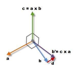
利用向量的三重积公式展开，且a.a = |a| = 1：
b’ = c x a = (a x b) x a = –a (a.b) + b(a.a) = b – a (a.b) = b + d，其中d = – a (a.b)是校正量，平行于a，方向取决于a和b的夹角。
上面的情况是a向量固定，b向量得到校正，下面分析对称的情况，a得到校正，b固定：
a’ = a – b (b.a) = a – b (a.b) = a + e，其中e = – b (a.b)
再下面考虑这两个向量都有误差，都得到一半的校正得：
a’ = a – b (a.b) / 2
b’ = b – a (a.b) / 2
所以得到一个相对简单的公式：
Err = (a.b)/2
a’ = a – Err b
b’ = b – Err a
现在我们可以更新DCM矩阵的 IB1, JB1向量。
Err = ( I$^B$$_1$ . J$^B$$_1$ ) / 2
I$^B$$_1$’ = I$^B$$_1$ – Err J$^B$$_1$
J$^B$$_1$’ = J$^B$$_1$ – Err I$^B$$_1$
I$^B$$_1$’’ = Normalize[I$^B$$_1$’]
J$^B$$_1$’’ = Normalize[J$^B$$_1$’]
K$^B$$_1$’’ = I$^B$$_1$’’ x J$^B$$_1$’’
其中Normalize[a] = a / |a|，单位化。

代码如下：

//bring dcm matrix in order - adjust values to make orthonormal (or at least closer to orthonormal)
void dcm_orthonormalize(float dcm[3][3]){
	//err = X . Y ,  X = X - err/2 * Y , Y = Y - err/2 * X  (DCMDraft2 Eqn.19)
	float err = vector3d_dot((float*)(dcm[0]),(float*)(dcm[1]));
	float delta[2][3];
	vector3d_scale(-err/2,(float*)(dcm[1]),(float*)(delta[0]));
	vector3d_scale(-err/2,(float*)(dcm[0]),(float*)(delta[1]));
	vector3d_add((float*)(dcm[0]),(float*)(delta[0]),(float*)(dcm[0]));
	vector3d_add((float*)(dcm[1]),(float*)(delta[1]),(float*)(dcm[1]));

	//Z = X x Y  (DCMDraft2 Eqn. 20) , 
	vector3d_cross((float*)(dcm[0]),(float*)(dcm[1]),(float*)(dcm[2]));
	//re-nomralization
	vector3d_normalize((float*)(dcm[0]));
	vector3d_normalize((float*)(dcm[1]));
	vector3d_normalize((float*)(dcm[2]));
}

DCM理论

注意：这部分属于APM源码里px4姿态解算部分。
资料翻译解读自DMCDraft2.pdf（翻译不妥请谅解，欢迎提意见，另外该理论文档已启动翻译，如果你想参与请点击这里），并结合文档分析了APM的姿态源码部分，目前还有drift_correction函数未进行整理！

前言

使用矩阵来控制和导航，元素包括陀螺仪，加速度计和gps信息。
总的来说，DCM工作如下：
- 陀螺仪作为主要的方向信息来源，通过整合一个非线性微分运动方程，表明飞机方向的变化率与旋转速率及它当前的方向之间的关系。
- 意识到积分过程中的积分误差将渐渐的违反DCM必须满足的正交约束，我们对矩阵的元素进行规则的小调整满足约束。
- 由于数字误差，陀螺仪漂移，陀螺仪偏移量将逐渐积累在DCM中的元素的误差，我们使用参考向量来检测误差，以及在检测到的误差和和第一步的陀螺仪输入中加一个比例积分负反馈控制器来在建立之前消除误差。gps是用来检测偏航误差，加速度计被用来检测俯仰和滚动。
  整个过程如下：
  
  代码实现概览：
  1
  2
  3
  4
  5
  6
  7
  8
  // Integrate the DCM matrix using gyro inputs
  matrix_update(delta_t);
  
  // Normalize the DCM matrix
  normalize();
  
  // Perform drift correction
  drift_correction(delta_t);

方向余弦矩阵介绍

所有这一切都与旋转有关。
有几种方法可以做到，比如旋转矩阵和四元数。这两种方法在实现上具有相似的地方，都是尽量准确的表示旋转。四元数只需要4个值，而旋转矩阵需要9个，在这方面四元数具有优势。而旋转矩阵很适合用来导航和控制。
旋转矩阵用来描述一个坐标系相对于另一个坐标系的方向。在一个系统中的向量可以通过乘以旋转矩阵转变到另一个系统中，如果是相反方向旋转则乘以旋转矩阵的逆矩阵，也是它的转置（交换行和列）。单位向量在控制和导航运算中将非常有用，因为它们的长度为1。因此他们能被用于交积和叉积中来获得各种正弦或余弦角。
随着飞机的飞行，我们可以用位置（重心的移动）和朝向（绕着重心方向的变化）了描述它的运动，类似这种变换我们称为刚体变换。通过指定一个轴的旋转来描述其相对于地球的方向。例如将飞机开始放在一个标准方向，然后将其旋转，它将指向另外一个实际的方向，也就是说任何其他的方向都可以通过标准方向的旋转描述。
旋转组是所有可能的旋转的组。它被称为一组，因为在该组中的任何2个旋转可以组成一个组中的另一个旋转，每一个旋转有一个逆旋转。这里有一个单位旋转。
旋转组应该得到重视的原因是，你能通过最少的近似来在各个方向控制和导航飞机，包括各种特技。
基本的想法是，定义了你的飞机的方向的旋转矩阵，可以通过结合描述旋转运动学的非线性微分方程得到。这个结合可以通过一系列的旋转组合完成，也就是两矩阵相乘，这是两个矩阵依次执行的结果。
然而，数值积分引入的数值误差，并不会产生与符号积分相同的结果。精确的陀螺仪信号的符号积分将产生完全正确的旋转矩阵。数值积分，即使我们有精确的陀螺仪信号，也会引入2种数值误差：
- 积分误差。数值积分采用有限时间步长和在有限采样速率下采样数据。因为是假定在时间步长内旋转速度是恒定的，这将引入了一个与旋转加速度成比例的误差。
- 量化误差。不管你用什么代表值，数字表示是有限的，所以有一个量化误差，从模数转换开始，以及所有计算没有保留结果所有位时。
旋转矩阵的一个关键特性是它的正交性，这意味着如果2个向量在一个参照系中是垂直的，它们在每一个参照系中都是垂直的。另外，在每一个参照系中向量的长度是一样的。数值误差可能违反此特性。在许多空间系统中,利用方向余弦矩阵把矢量从一个笛卡尔坐标系变换到另一个笛卡尔坐标系。理想的方向余弦矩阵应当是正交的,而实际上,通过计算得到的矩阵由于种种误差(如计算方法误差、舍入误差等)而失去了正交性,造成变换误差,影响系统精度。于是有必要按某种最优方式,恢复其正交性。矩阵正交化的迭代法有多种,但都计算较繁、运算量大。对于需要把计算得到的方向余弦矩阵周期性地正交化的场合(如捷联式惯导系统),大的运算量将给计算机实时计算带来困难。例如，即使行和列都应该代表单位向量，它们的大小应该等于1，但数值误差可能导致它们变得更小或更大。最终他们可以缩小到零，或去无限。行和列应该是垂直于彼此，数值误差可能导致他们“倾斜”到对方，如下图所示：
旋转矩阵有9个元素。实际上，只有3个是独立的。旋转矩阵的正交特性在数学术语方面意味着矩阵的任何一对行或列都是垂直的。并且在每个列（或行）的元素的平方和等于1。所以这九个元素中有六个约束条件。
反对称矩阵定义是：A=-A’（A的转置前加负号），它的第Ⅰ行和第Ⅰ列各数绝对值相等，符号相反。且主对角线上的元素为均为零。一个小的旋转可以用如下的反对称矩阵来描述：
在我们的例子中，运动学与刚体旋转的含义有关。它的结果是一个非线性微分方程，描述了刚体在其向量旋转速度方面的时间演化。方向余弦矩阵都是关于运动学的。
控制和导航可以在笛卡尔坐标系使用DCM完成叉积和点积运算。下面是具体步骤：
- 要控制飞机的俯仰，你需要知道这架飞机的俯仰姿态，你可以通过把飞机的翻滚轴与地面垂直做点积。
- 要控制飞机的翻滚，你需要知道这架飞机的倾斜姿态，你可以通过把飞机的俯仰轴与地面垂直做点积。
- 要航向，你需要知道你这架飞机相对于你想要去的方向的偏航姿态，可以通过飞机的翻滚轴与想要去的方向的向量做叉积得到。如果是去相反的方向，则是点积运算。
- 判断飞机是否倒过来，可以通过判断飞机偏航轴与垂直的点积符号，如果小于0，则是朝下的。
- 计算飞机绕垂直轴的旋转速度，将陀螺仪的旋转矢量转换为地理参考坐标系，然后与垂直轴做点积。
下面将进行深入的理论研究。
确定一个合适的坐标系统描述飞机的运动是必要的。对于大多数处理飞机运动的问题，采用了双坐标系。一个坐标系是固定在地球上的，可以被认为是是一个惯性坐标系，是为了飞机运动分析的目的。另一个坐标系是固定在飞机上的，被称为机体坐标系。图2显示了两右手坐标系：

其中 xe、ye、ze 是地球坐标系统,ze 指向地心,xe 指向正东方,ye 指向正北方;
xb、yb、zb 为机体坐标系。
飞机的方向经常被描述为三个连续的旋转，其顺序是重要的。旋转角被称为欧拉角。假设机体坐标如下：

进行如下的旋转就可以得到上面图2的结果：

分析：第一步:假设我站在机体坐标中,我需要通过先绕 Xb 轴旋转 $\Phi$ ，再旋转 Yb 轴旋转 $\theta$，最后绕 Zb 轴旋转 $\psi$，回到地球坐标系;先求出每次旋转的矩阵。
如果绕机体 X 轴旋转的角度为 $\Phi$，那么

这里是怎么得来的呢？先说一下什么是旋转矩阵？如下图所示，我们假设最开始空间的坐标系也就是机体坐标系X$_A$，Y$_A$，Z$_A$就是笛卡尔坐标系，这样我们得到空间A的矩阵V$_A$={X$_A$，Y$_A$，Z$_A$}$^T$，其实也可以看做是单位阵E。进过旋转后，空间A的三个坐标系变成了图1中红色的三个坐标系X$_B$，Y$_B$，Z$_B$，得到空间B的矩阵V$_B$={X$_B$，Y$_B$，Z$_B$}$^T$。我们将两个空间联系起来可以得到V$_B$=R•V$_A$，这里R就是我们所说的旋转矩阵。

由于X$_A$={1,0,0}$^T$，Y$_A$={0,1,0}$^T$，Z$_A$={0,0,1}$^T$，结合下图可以看出，旋转矩阵R就是由X$_B$，Y$_B$，Z$_B$ 三个向量组成的。讲到这里，大家应该会发现旋转矩阵R满足第一个条件，因为单位向量无论怎么旋转长度肯定不会变而且向量之间的正交性质也不会变。那么旋转矩阵就是正交阵！不过这还不能说明问题，下面我更进一步利用数学公式进行证明。

进一步讨论之前，我们先说两点数学知识。（1）点乘（dot product）的几何意义：如下图，我们从点乘的公式可以得到α•β相当于β的模乘上α在β上投影的模，所以当|β|=1时，α•β就是指α在β上投影的模。这一点在下面的内容中非常重要，之所以叫余弦矩阵的原因就是这个。（2）旋转矩阵逆的几何意思：这个比较抽象，不过也好理解。旋转矩阵相当于把一个向量（空间）旋转成新的向量（空间），那么逆可以理解为由新的向量（空间）转回原来的向量（空间）。（3）向量是特殊的矩阵，只有一行或一列的矩阵称为向量。向量有叉乘和点乘。矩阵也有，但意义不一样，矩阵还有反对称，逆矩阵等。

所以上面的公式解析如下：

同理，其他方向的旋转计算如下：
如果绕机体 Y 轴旋转的角度为 $\theta$，那么

如果绕机体 Z 轴旋转的角度为 $\psi$，那么

第二步:由于站在机体坐标上需要按照 X->Y->Z 轴的顺序,经过 3 次旋转,才能回到地球坐标系;反过来如果站在地球坐标系,则需要经过 Z->Y->X 的三次旋转才能到达机体坐标系。因此我们可以列出从地球坐标系到机体坐标系的DCM矩阵，换句话说此DCM矩阵就是机体坐标在地理坐标系中的表示，其中$\Phi, \theta, \psi$为机体在地理坐标系中的姿态角。
$$L(\Phi, \theta, \psi) = L(\psi) L(\theta) L(\Phi);$$
矩阵的乘法计算得：
方向余弦矩阵：向量的某些类型，如方向，速度，加速度，和转换，（动作）可以转化为旋转参考系中的一个3x3的矩阵。我们感兴趣的是机体参考系和地面参考系。它可以乘以一个向量的方向余弦矩阵旋转：
由上面的分析可知，方向余弦矩阵与欧拉角之间的关系为：

方程1方程2表明了如何将机体坐标系中测得的向量转换的地理坐标系中。方程1是以方向余弦角的形式，而2为欧拉角。

以上整个求解过程是对 matrix3.cpp 代码中 from_euler 函数的解析：

// create a rotation matrix given some euler angles
// this is based on http://gentlenav.googlecode.com/files/EulerAngles.pdf
template <typename T>
void Matrix3<T>::from_euler(float roll, float pitch, float yaw)
{
    float cp = cosf(pitch);//pitch 表示俯仰相对于地球坐标系的角度值
    float sp = sinf(pitch);
    float sr = sinf(roll);//roll 表示横滚相对于地球坐标系的角度值
    float cr = cosf(roll);
    float sy = sinf(yaw);//yaw 表示偏航相对于地球坐标的角度值
    float cy = cosf(yaw);

    a.x = cp * cy;
    a.y = (sr * sp * cy) - (cr * sy);
    a.z = (cr * sp * cy) + (sr * sy);
    b.x = cp * sy;
    b.y = (sr * sp * sy) + (cr * cy);
    b.z = (cr * sp * sy) - (sr * cy);
    c.x = -sp;
    c.y = sr * cp;
    c.z = cr * cp;
}

其中a，b，c为类定义的私有变量—向量。
通过不同的旋转顺序可以得到不同的旋转矩阵，如果从地球坐标系到体坐标系,按照 Z->X->Y 轴的顺序旋转可以得到from_euler312函数，这里就没做具体讲解。

问题：反过来也就可以通过方向余弦矩阵来求出旋转角

函数 to_euler 式通过上面的 3 个公式求出对应的角度的

// calculate euler angles from a rotation matrix
// this is based on http://gentlenav.googlecode.com/files/EulerAngles.pdf
template <typename T>
void Matrix3<T>::to_euler(float *roll, float *pitch, float *yaw) const
{
    if (pitch != NULL) {
        *pitch = -safe_asin(c.x);
    }
    if (roll != NULL) {
        *roll = atan2f(c.y, c.z);
    }
    if (yaw != NULL) {
        *yaw = atan2f(b.x, a.x);
    }
}

地理坐标系中向量的每个分量等于相对应的旋转矩阵的行与机体坐标向量的点积。计算旋转矩阵需要9个乘法和6个加法运算。方程3是方程1的复述，用乘法展开向量和矩阵的元素。所以如果知道机体坐标向量，即可得地理坐标向量的大小：
需要注意的是，矩阵R不一定是对称的。R矩阵的三列对应于机体坐标的三个轴向量到地理坐标的变换。R矩阵的三行则对应于地理坐标三个轴向量到机体坐标的变换。该R矩阵描述了所有机体相对于地球方向的信息。R矩阵也称为方向余弦矩阵，因为每个分量都是机体坐标轴与地理坐标轴夹角的余弦，通过看推理余弦矩阵部分可以看出来。
矩阵的转置，特别在旋转矩阵中，表示为$R^T$，通过交换行和列得到。一般来说，一个方形矩阵的逆矩阵如果存在的话，表示为$R^{−1}$。矩阵的逆乘以矩阵得到的是单位矩阵。（单位矩阵就是对角线上元素为1,其余为0,单位矩阵乘以任何矩阵得到它本身），对于旋转矩阵来说，逆就等于它的转置。
之所以旋转矩阵逆就等于它的转置考虑到了对称性的情况。旋转矩阵的元素都是机体轴与地理坐标轴之间的余弦值，相反的情况就相当于交换地理坐标和机体坐标的角色，也就是说交换行与列，这跟转置是一样的。实际上这又和正交条件达成一致：
- 正交矩阵每一列都是单位矩阵，并且两两正交。最简单的正交矩阵就是单位阵。
- 正交矩阵的逆（inverse）等于正交矩阵的转置（transpose）。同时可以推论出正交矩阵的行列式的值肯定为正负1的。
- 正交矩阵满足很多矩阵性质，比如可以相似于对角矩阵等等。
  
  如下：
  
  这个方程用来证明矩阵的逆的矩阵的转置。
旋转矩阵的一个非常有用的特性是，我们可以组成旋转。

这里特别需要小心运算顺序，因为它的效果是完全不一样的。
另外这里还有一些有用的特性，如：
下面介绍一下点乘和叉乘。
这里有两个DCM计算里边用到的向量运算——点乘和叉乘。点乘是表量运算，A向量作为行向量，B向量作为列向量。

可以证明向量的点乘等于两个向量的长度乘以它们角度的余弦值。

所以向量的点乘是对称的。A $\cdot$ B = B $\cdot$ A

而两个向量的叉乘是一个向量。它的元素是这样计算的：

从物理意义上来分析：

所以叉乘是反对称的，A $\times$ B = - B $\times$ A

方向余弦矩阵的更新

下面到了DCM算法的核心部分——由陀螺仪计算方向余弦矩阵。
核心概念：非线性微分方程——方向余弦的变化速率与陀螺仪之间的关系。我们的目标是计算方向余弦而不是任何违反方程非线性的近似解。目前，我们假设陀螺仪信号没有错误。稍后我们将解决陀螺仪漂移问题。
不像机械陀螺，我们不能通过简单地积分陀螺仪信号得到角度。一个有名的运动学公式，关于旋转向量的变化率和它的旋转之间的关系：

下面解释一下这个公式，如下图所示，r为任意的旋转向量，t时刻的坐标为r(t)。时间间隔dt后：r = r (t) , r’= r (t+dt) and dr = r’ – r。
dt时间后向量r绕着与单位向量u同向的轴旋转了d$\theta$，停到了向量r’的位置。其中u垂直与旋转的机身，因此u正交于r与r’，图中显示了u与u’，它们与r和r‘的叉乘结果方向相同。故有
u = (r x r’) / |r x r’| = (r x r’) / (|r|| r’|sin(dθ)) = (r x r’) / (|r|2 sin(dθ))
由于旋转并不改变向量的长度，因此有| r’| = |r|。
向量r的线速度可以表示如下：
v = dr / dt = ( r’ – r) / dt
v = w x r
故可以得出上面的公式。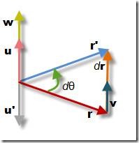

有一个需要注意的地方：
- 微分方程是非线性的。旋转向量输入是与我们要进行积分的变量进行叉乘。因此，任何线性的方法都只是一种近似。
- 两个向量都应该在同一个坐标系中测量。
- 因为叉乘是不对称的，所以我们需要保存结果，然后改变它的方向。

如果知道了初始状态和旋转向量的时间，我们可以通过方程11的数值积分来跟踪旋转向量。

将方程13用于R矩阵的行或列中，可看作成旋转向量。
这里遇到的第一个问题是，我们要跟踪的向量和旋转向量不是在同一坐标系做测量的。理想情况下，我们都是在地理坐标轴中跟踪机体坐标轴，但是陀螺仪是在机体坐标中测量的。一个简单的方法是通过对称性解决，地理坐标在机体坐标中旋转和机体坐标在地理坐标中旋转是相反的，所以只要改变陀螺仪的符号就好了，更加方便的方法是，交换叉乘的顺序就好了。

这里的向量代表的是方程1中R矩阵的行。下面的问题是怎么实施方程14，回归到方程14的微分方程形式：

由这里可知方向余弦矩阵R的行都是通过$r_{earth}(t) \times d\theta(t)$积分得到的。
所以根据陀螺仪的角度值,来计算当前机体的姿态 DCM矩阵，其使用的方法是：机体坐标的每个轴的向量与 g(陀螺仪改变的角度向量)求叉积，这里求的是角度改变后,姿态在各个方向上的变化量，所以最后使用了矩阵的加法。源码matrix3.cpp中的函数体现如下：

// apply an additional rotation from a body frame gyro vector
// to a rotation matrix.
template <typename T>
void Matrix3<T>::rotate(const Vector3<T> &g)
{
    Matrix3<T> temp_matrix;
    temp_matrix.a.x = a.y * g.z - a.z * g.y;
    temp_matrix.a.y = a.z * g.x - a.x * g.z;
    temp_matrix.a.z = a.x * g.y - a.y * g.x;
    temp_matrix.b.x = b.y * g.z - b.z * g.y;
    temp_matrix.b.y = b.z * g.x - b.x * g.z;
    temp_matrix.b.z = b.x * g.y - b.y * g.x;
    temp_matrix.c.x = c.y * g.z - c.z * g.y;
    temp_matrix.c.y = c.z * g.x - c.x * g.z;
    temp_matrix.c.z = c.x * g.y - c.y * g.x;

    (*this) += temp_matrix;
}

还有一件事需要做，陀螺仪漂移将在后面进行。我们需要通过比例积分补偿反馈控制器来添加旋转速率校准到陀螺仪测量的数据上，以此产生最优的角速率估计。

基本上，我们的GPS和加速度计的参考向量被用来计算旋转误差，并通过反馈控制器输入计算，然后更新原有计算。

我们可以把方程15转化为矩阵的形式，这里推导有点复杂，可以了解下矢量阵或者summer的文章，如下：

方程17就是从陀螺仪信号更新方向余弦矩阵，其对角线上的1就为方程15的第一个条目，其余的为第二个条目，这种方法是用矩阵的乘法实现的，它包含27个乘法和18个加法。正好适合dsPIC30F4011，因为它支持矩阵乘法运算，如果芯片不支持，也可以用方程15的积分形式实现。故在apm里采用的是积分形式累加的。矩阵更新的源码体现如下：

// update the DCM matrix using only the gyros
void
AP_AHRS_DCM::matrix_update(float _G_Dt)
{
    // note that we do not include the P terms in _omega. This is
    // because the spin_rate is calculated from _omega.length(),
    // and including the P terms would give positive feedback into
    // the _P_gain() calculation, which can lead to a very large P
    // value
    _omega.zero();

    // average across first two healthy gyros. This reduces noise on
    // systems with more than one gyro. We don't use the 3rd gyro
    // unless another is unhealthy as 3rd gyro on PH2 has a lot more
    // noise
    uint8_t healthy_count = 0;
    Vector3f delta_angle;
    for (uint8_t i=0; i<_ins.get_gyro_count(); i++) {
        if (_ins.get_gyro_health(i) && healthy_count < 2) {
            Vector3f dangle;
            if (_ins.get_delta_angle(i, dangle)) {
                healthy_count++;
                delta_angle += dangle;
            }
        }
    }
    if (healthy_count > 1) {
        delta_angle /= healthy_count; //获取角度变化量
    }
    if (_G_Dt > 0) {
        _omega = delta_angle / _G_Dt;
        _omega += _omega_I;
        _dcm_matrix.rotate((_omega + _omega_P + _omega_yaw_P) * _G_Dt); //将角度变化量与旋转向量进行叉乘，然后累加
    }
}

再归一化重整

由于上述的公式是在dt非常小的情况下才误差比较小，这种数字误差将驱使方程4的正交条件逐渐不满足，导致坐标系的两个轴不再能描述刚体。值得幸运的是，数字误差累加的很慢，我们完全可以提前采取办法解决它。
我们将这种解决办法称为归一化，我们设计了几种方法，模拟实现都可行，最后选择了一种最优的方法。
首先计算矩阵列向量X、Y的点乘，理论上应该等于0，所以它的结果可以看出向量偏了多少。

将这个误差平分到X、Y向量：

可以将方程19代人方程18中，验证正交性误差大大减少了。记住R矩阵的行与列的范数为1，将误差平分给两个轴比只分个一个产生较低的残余误差。
下一步就是调整Z列向量正交于X和Y。这个很简单，只要进行叉乘就可以了：

最后一步为，确保R矩阵的各列向量的模为1，一种方法可以通过平方根来求，但是这里有一种更加简单的办法，考虑到这个模不会与1有太大差别，这里可以使用泰勒展开。

方程21做的事情就是调整各列向量的模为1。展开为3减去向量模的平方，乘以1/2，再乘以这个向量。所以计算更加简单。
源码实现如下：

/*************************************************
	-  Direction Cosine Matrix IMU: Theory
	-  William Premerlani and Paul Bizard
 *
	-  Numerical errors will gradually reduce the orthogonality conditions expressed by equation 5
	-  to approximations rather than identities. In effect, the axes in the two frames of reference no
	-  longer describe a rigid body. Fortunately, numerical error accumulates very slowly, so it is a
	-  simple matter to stay ahead of it.
	-  We call the process of enforcing the orthogonality conditions ÒrenormalizationÓ.
 */
void
AP_AHRS_DCM::normalize(void)
{
    float error;
    Vector3f t0, t1, t2;

    error = _dcm_matrix.a * _dcm_matrix.b;                                              // eq.18

    t0 = _dcm_matrix.a - (_dcm_matrix.b * (0.5f * error));              // eq.19
    t1 = _dcm_matrix.b - (_dcm_matrix.a * (0.5f * error));              // eq.19
    t2 = t0 % t1;                                                       // c= a x b // eq.20

    if (!renorm(t0, _dcm_matrix.a) ||
            !renorm(t1, _dcm_matrix.b) ||
            !renorm(t2, _dcm_matrix.c)) {
        // Our solution is blowing up and we will force back
        // to last euler angles
        _last_failure_ms = AP_HAL::millis();
        AP_AHRS_DCM::reset(true);
    }
}

// renormalise one vector component of the DCM matrix
// this will return false if renormalization fails
bool
AP_AHRS_DCM::renorm(Vector3f const &a, Vector3f &result)
{
    float renorm_val;

    // numerical errors will slowly build up over time in DCM,
    // causing inaccuracies. We can keep ahead of those errors
    // using the renormalization technique from the DCM IMU paper
    // (see equations 18 to 21).

    // For APM we don't bother with the taylor expansion
    // optimisation from the paper as on our 2560 CPU the cost of
    // the sqrt() is 44 microseconds, and the small time saving of
    // the taylor expansion is not worth the potential of
    // additional error buildup.

    // Note that we can get significant renormalisation values
    // when we have a larger delta_t due to a glitch eleswhere in
    // APM, such as a I2c timeout or a set of EEPROM writes. While
    // we would like to avoid these if possible, if it does happen
    // we don't want to compound the error by making DCM less
    // accurate.

    renorm_val = 1.0f / a.length(); //这里并没有使用泰勒展开，考虑的节省的时间不多

    // keep the average for reporting
    _renorm_val_sum += renorm_val;
    _renorm_val_count++;

    if (!(renorm_val < 2.0f && renorm_val > 0.5f)) {
        // this is larger than it should get - log it as a warning
        if (!(renorm_val < 1.0e6f && renorm_val > 1.0e-6f)) {
            // we are getting values which are way out of
            // range, we will reset the matrix and hope we
            // can recover our attitude using drift
            // correction before we hit the ground!
            //Serial.printf("ERROR: DCM renormalisation error. renorm_val=%f\n",
            //	   renorm_val);
            return false;
        }
    }

    result = a * renorm_val;
    return true;
}

EKF设计与实现

资料搜集

APM的EKF源码流分析：
ArduCopter.cpp里fast_loop函数里的姿态更新部分如下：

void AP_AHRS_NavEKF::update(void)
{
    update_DCM();
    update_EKF1();
    update_EKF2();
#if CONFIG_HAL_BOARD == HAL_BOARD_SITL
    update_SITL();
#endif
}

这里看出姿态估算使用了DCM和EKF算法，而EKF由分为两种，第一种为默认推荐的稳定版代码飞行的，第二种为git上master的，是另外一种形式的升级版EKF，这种EKF可以通过一个移动的平台起飞。下面以master版本分析，具体解释如下：

void AP_AHRS_NavEKF::update_EKF2(void) //master版（即开发版）实验表明，最后是由这个函数生成的姿态角
{
    if (!ekf2_started) {
        // wait 1 second for DCM to output a valid tilt error estimate
        if (start_time_ms == 0) {
            start_time_ms = AP_HAL::millis();
        }
        if (AP_HAL::millis() - start_time_ms > startup_delay_ms) {
            ekf2_started = EKF2.InitialiseFilter(); //使用了DCM的_error_rp = 0.8f * _error_rp + 0.2f * best_error;，来源drift_correction，所以EKF依赖于DCM
        }
    }
    if (ekf2_started) {
        EKF2.UpdateFilter();
        if (active_EKF_type() == EKF_TYPE2) {
            Vector3f eulers;
            EKF2.getRotationBodyToNED(_dcm_matrix); ////这里的矩阵重新赋值了DCM矩阵，即姿态
            EKF2.getEulerAngles(-1,eulers);
            roll  = eulers.x; //生成roll
            pitch = eulers.y;
            yaw   = eulers.z;

            update_cd_values(); //生成roll_sensor
            update_trig(); //生成_cos_roll

            // keep _gyro_bias for get_gyro_drift()
            EKF2.getGyroBias(-1,_gyro_bias);
            _gyro_bias = -_gyro_bias;

            // calculate corrected gryo estimate for get_gyro()
            _gyro_estimate.zero();
            uint8_t healthy_count = 0;
            for (uint8_t i=0; i<_ins.get_gyro_count(); i++) {
                if (_ins.get_gyro_health(i) && healthy_count < 2) {
                    _gyro_estimate += _ins.get_gyro(i);
                    healthy_count++;
                }
            }
            if (healthy_count > 1) {
                _gyro_estimate /= healthy_count;
            }
            _gyro_estimate += _gyro_bias;

            float abias;
            EKF2.getAccelZBias(-1,abias);

            // This EKF uses the primary IMU
            // Eventually we will run a separate instance of the EKF for each IMU and do the selection and blending of EKF outputs upstream
            // update _accel_ef_ekf
            for (uint8_t i=0; i<_ins.get_accel_count(); i++) {
                Vector3f accel = _ins.get_accel(i);
                if (i==_ins.get_primary_accel()) {
                    accel.z -= abias;
                }
                if (_ins.get_accel_health(i)) {
                    _accel_ef_ekf[i] = _dcm_matrix * accel;
                }
            }
            _accel_ef_ekf_blended = _accel_ef_ekf[_ins.get_primary_accel()];
        }
    }
}

概要：在这个函数里有一个active_EKF_type()函数，通过分析可知它的值为EKF_TYPE2，故使用的是EKF2算法。具体分析如下

AP_AHRS_NavEKF::EKF_TYPE AP_AHRS_NavEKF::active_EKF_type(void) const
{
    EKF_TYPE ret = EKF_TYPE_NONE;
/*
    enum EKF_TYPE {EKF_TYPE_NONE=0,
                   EKF_TYPE1=1,
                   EKF_TYPE2=2
#if CONFIG_HAL_BOARD == HAL_BOARD_SITL
                   ,EKF_TYPE_SITL=10
#endif
    };
*/
    switch (ekf_type()) {
    case 0:
        return EKF_TYPE_NONE;

    case 1: { 
        // do we have an EKF yet?
        if (!ekf1_started) {
            return EKF_TYPE_NONE;
        }
        if (always_use_EKF()) {
/*
    bool always_use_EKF() const {
        return _ekf_flags & FLAG_ALWAYS_USE_EKF; //下面分析这两个数据,结果为0
    }

// constructor
AP_AHRS_NavEKF::AP_AHRS_NavEKF(AP_InertialSensor &ins, AP_Baro &baro, AP_GPS &gps, RangeFinder &rng,
                               NavEKF &_EKF1, NavEKF2 &_EKF2, Flags flags) :
    AP_AHRS_DCM(ins, baro, gps),
    EKF1(_EKF1),
    EKF2(_EKF2),
    _ekf_flags(flags)
{
    _dcm_matrix.identity();
}

enum Flags {
        FLAG_NONE = 0,
        FLAG_ALWAYS_USE_EKF = 0x1, //FLAG_ALWAYS_USE_EKF = 0x1
    };

    // Constructor
    AP_AHRS_NavEKF(AP_InertialSensor &ins, AP_Baro &baro, AP_GPS &gps, RangeFinder &rng,
                   NavEKF &_EKF1, NavEKF2 &_EKF2, Flags flags = FLAG_NONE); //所以_ekf_flags = FLAG_NONE = 0
*/
        	uint8_t ekf_faults;
            EKF1.getFilterFaults(ekf_faults);
            if (ekf_faults == 0) {
                ret = EKF_TYPE1;
            }
        } else if (EKF1.healthy()) {
            ret = EKF_TYPE1;
        }
        break;
    }

    case 2: { //由下面的函数分析可知，应该会跳到这里
        // do we have an EKF2 yet?
        if (!ekf2_started) {
            return EKF_TYPE_NONE;
        }
        if (always_use_EKF()) {
            uint8_t ekf2_faults;
            EKF2.getFilterFaults(-1,ekf2_faults);
            if (ekf2_faults == 0) {
                ret = EKF_TYPE2;
            }
        } else if (EKF2.healthy()) {
            ret = EKF_TYPE2; //最终的返回结果
        }
        break;
    }

#if CONFIG_HAL_BOARD == HAL_BOARD_SITL
    case EKF_TYPE_SITL:
        ret = EKF_TYPE_SITL;
        break;
#endif
    }

    /*
      fixed wing and rover when in fly_forward mode will fall back to
      DCM if the EKF doesn't have GPS. This is the safest option as
      DCM is very robust
     */
    if (ret != EKF_TYPE_NONE &&
        (_vehicle_class == AHRS_VEHICLE_FIXED_WING ||
         _vehicle_class == AHRS_VEHICLE_GROUND) &&
        _flags.fly_forward) {
        nav_filter_status filt_state;
        if (ret == EKF_TYPE1) {
            EKF1.getFilterStatus(filt_state);
#if CONFIG_HAL_BOARD == HAL_BOARD_SITL
        } else if (ret == EKF_TYPE_SITL) {
            get_filter_status(filt_state);
#endif
        } else {
            EKF2.getFilterStatus(-1,filt_state);
        }
        if (hal.util->get_soft_armed() && !filt_state.flags.using_gps && _gps.status() >= AP_GPS::GPS_OK_FIX_3D) {
            // if the EKF is not fusing GPS and we have a 3D lock, then
            // plane and rover would prefer to use the GPS position from
            // DCM. This is a safety net while some issues with the EKF
            // get sorted out
            return EKF_TYPE_NONE;
        }
        if (hal.util->get_soft_armed() && filt_state.flags.const_pos_mode) {
            return EKF_TYPE_NONE;
        }
        if (!filt_state.flags.attitude ||
                !filt_state.flags.horiz_vel ||
                !filt_state.flags.vert_vel ||
                !filt_state.flags.horiz_pos_abs ||
                !filt_state.flags.vert_pos) {
            return EKF_TYPE_NONE;
        }
    }
    return ret;
}

其中又涉及到了ekf_type函数，可知返回值为2：

//canonicalise _ekf_type, forcing it to be 0, 1 or 2

uint8_t AP_AHRS_NavEKF::ekf_type(void) const
{
    uint8_t type = _ekf_type; //由下面的分析，默认_ekf_type的值为2
    if (always_use_EKF() && type == 0) { //如果总是使用EKF且默认type为0时，那么type就强制为1
        type = 1;
    }

//  bool always_use_EKF() const {
//      return _ekf_flags & FLAG_ALWAYS_USE_EKF; //位运算，结果为0
//  }

    // check for invalid type
#if CONFIG_HAL_BOARD == HAL_BOARD_SITL
    if (type > 2 && type != EKF_TYPE_SITL) { //检查type是否有效，只有为SIL的时候才能大于2
        type = 1;
    }
#else
    if (type > 2) {
        type = 1;
    }
#endif
    return type;
}

_ekf_type的默认取值分析。

#if AP_AHRS_NAVEKF_AVAILABLE //_ekf_type的默认取值为2
    // @Param: EKF_TYPE
    // @DisplayName: Use NavEKF Kalman filter for attitude and position estimation
    // @Description: This controls whether the NavEKF Kalman filter is used for attitude and position estimation and whether fallback to the DCM algorithm is allowed. Note that on copters "disabled" is not available, and will be the same as "enabled - no fallback"
    // @Values: 0:Disabled,1:Enabled,2:Enable EKF2
    // @User: Advanced
    AP_GROUPINFO("EKF_TYPE",  14, AP_AHRS, _ekf_type, 2),
#endif

在DCM算法里，与ekf算法一样，最后都生成了roll, roll_sensor， _cos_roll。

// calculate the euler angles and DCM matrix which will be used for high level
// navigation control. Apply trim such that a positive trim value results in a
// positive vehicle rotation about that axis (ie a negative offset)
void
AP_AHRS_DCM::euler_angles(void)
{
    _body_dcm_matrix = _dcm_matrix;
    _body_dcm_matrix.rotateXYinv(_trim);
    _body_dcm_matrix.to_euler(&roll, &pitch, &yaw);

    update_cd_values();
}

/*
  update the centi-degree values
 */
void AP_AHRS::update_cd_values(void)
{
    roll_sensor  = degrees(roll) * 100;
    pitch_sensor = degrees(pitch) * 100;
    yaw_sensor   = degrees(yaw) * 100;
    if (yaw_sensor < 0)
        yaw_sensor += 36000;
}

// update trig values including _cos_roll, cos_pitch
update_trig();

EKF1与EKF2的切换：这里假设你自己在开发版代码中想使用EKF1怎么办？
直接进行参数配置或者在地面站修改EKF相关的参数即可，具体如下修改即可

源码修改，全局搜索到如下地方，更改成下面的样子。

1
2
3

AP_GROUPINFO_FLAGS("ENABLE", 0, NavEKF2, _enable, 0, AP_PARAM_FLAG_ENABLE),
AP_GROUPINFO_FLAGS("ENABLE", 34, NavEKF, _enable, 1, AP_PARAM_FLAG_ENABLE),
AP_GROUPINFO("EKF_TYPE",  14, AP_AHRS, _ekf_type, 1),

地面站也是要修改三个地方。

可以总结出各个参数都在各自的cpp文件中有默认值
如AP_MotorsMulticopter.cpp中的AP_GROUPINFO(“CURR_MAX”, 12, AP_MotorsMulticopter, _batt_current_max, AP_MOTORS_CURR_MAX_DEFAULT),设置解锁时电机的转速。

姿态控制

预习材料：PID参数调节/串级PID/串级PID1

下面将先进行APM源码自稳模式的PID数据流分析：
在AC_AttitudeControl.cpp里

void AC_AttitudeControl::attitude_controller_run_quat(const Quaternion& att_target_quat, const Vector3f& att_target_ang_vel_rads)
{
    // Update euler attitude target and angular velocity target
    att_target_quat.to_euler(_att_target_euler_rad.x,_att_target_euler_rad.y,_att_target_euler_rad.z); //将四元数的目标姿态角装换为欧拉角
    _att_target_ang_vel_rads = att_target_ang_vel_rads;

    // Retrieve quaternion vehicle attitude
    // TODO add _ahrs.get_quaternion()
    Quaternion att_vehicle_quat;
    att_vehicle_quat.from_rotation_matrix(_ahrs.get_rotation_body_to_ned()); //获得机体姿态角
    // Compute attitude error
    (att_vehicle_quat.inverse()*att_target_quat).to_axis_angle(_att_error_rot_vec_rad); //计算角度误差

    // Compute the angular velocity target from the attitude error
    update_ang_vel_target_from_att_error(); //内环P控制，更新_ang_vel_target_rads外环控制值

    // Add the angular velocity feedforward, rotated into vehicle frame
    Matrix3f Trv;
    get_rotation_reference_to_vehicle(Trv);
    _ang_vel_target_rads += Trv * _att_target_ang_vel_rads; //更新_ang_vel_target_rads外环控制值
}

其中get_rotation_body_to_ned函数的原型为：

const Matrix3f &AP_AHRS_NavEKF::get_rotation_body_to_ned(void) const
{
    if (!active_EKF_type()) { //如果没有使用EKF,则使用DCM算法生成的矩阵
        return AP_AHRS_DCM::get_rotation_body_to_ned();
    }
    return _dcm_matrix; //否则使用EKF2生成的矩阵
}

// return rotation matrix representing rotaton from body to earth axes
onst Matrix3f &get_rotation_body_to_ned(void) const {
    return _body_dcm_matrix;
}

另为，内环P控制，输出值_ang_vel_target_rads为外环PID目标控制值。

void AC_AttitudeControl::update_ang_vel_target_from_att_error()
{
    // Compute the roll angular velocity demand from the roll angle error
    if (_att_ctrl_use_accel_limit && _accel_roll_max > 0.0f) {
        _ang_vel_target_rads.x = sqrt_controller(_att_error_rot_vec_rad.x, _p_angle_roll.kP(), constrain_float(get_accel_roll_max_radss()/2.0f,  AC_ATTITUDE_ACCEL_RP_CONTROLLER_MIN_RADSS, AC_ATTITUDE_ACCEL_RP_CONTROLLER_MAX_RADSS));
    }else{
        _ang_vel_target_rads.x = _p_angle_roll.kP() * _att_error_rot_vec_rad.x;
    }

    // Compute the pitch angular velocity demand from the roll angle error
    if (_att_ctrl_use_accel_limit && _accel_pitch_max > 0.0f) {
        _ang_vel_target_rads.y = sqrt_controller(_att_error_rot_vec_rad.y, _p_angle_pitch.kP(), constrain_float(get_accel_pitch_max_radss()/2.0f,  AC_ATTITUDE_ACCEL_RP_CONTROLLER_MIN_RADSS, AC_ATTITUDE_ACCEL_RP_CONTROLLER_MAX_RADSS));
    }else{
        _ang_vel_target_rads.y = _p_angle_pitch.kP() * _att_error_rot_vec_rad.y;
    }

    // Compute the yaw angular velocity demand from the roll angle error
    if (_att_ctrl_use_accel_limit && _accel_yaw_max > 0.0f) {
        _ang_vel_target_rads.z = sqrt_controller(_att_error_rot_vec_rad.z, _p_angle_yaw.kP(), constrain_float(get_accel_yaw_max_radss()/2.0f,  AC_ATTITUDE_ACCEL_Y_CONTROLLER_MIN_RADSS, AC_ATTITUDE_ACCEL_Y_CONTROLLER_MAX_RADSS));
    }else{
        _ang_vel_target_rads.z = _p_angle_yaw.kP() * _att_error_rot_vec_rad.z;
    }

    // Add feedforward term that attempts to ensure that the copter yaws about the reference
    // Z axis, rather than the vehicle body Z axis.
    // NOTE: This is a small-angle approximation.
    _ang_vel_target_rads.x += _att_error_rot_vec_rad.y * _ahrs.get_gyro().z;
    _ang_vel_target_rads.y += -_att_error_rot_vec_rad.x * _ahrs.get_gyro().z;
}

外环PID控制并设置电机值。

void AC_AttitudeControl::rate_controller_run()
{
    _motors.set_roll(rate_bf_to_motor_roll(_ang_vel_target_rads.x));
    _motors.set_pitch(rate_bf_to_motor_pitch(_ang_vel_target_rads.y));
    _motors.set_yaw(rate_bf_to_motor_yaw(_ang_vel_target_rads.z));
}

这个函数位于ArduCopter.cpp里的fast_loop函数里，它是放于内环控制之前的。如下：

// Main loop - 400hz
void Copter::fast_loop()
{

    // IMU DCM Algorithm
    // --------------------
    read_AHRS();

    // run low level rate controllers that only require IMU data
    attitude_control.rate_controller_run(); //外环并赋值给电机
    
#if FRAME_CONFIG == HELI_FRAME
    update_heli_control_dynamics();
#endif //HELI_FRAME

    // send outputs to the motors library
    motors_output();

    // Inertial Nav
    // --------------------
    read_inertia();

    // check if ekf has reset target heading
    check_ekf_yaw_reset();

    // run the attitude controllers
    update_flight_mode(); //如果仅考虑自稳模式，内环控制在这个里边

    // update home from EKF if necessary
    update_home_from_EKF();

    // check if we've landed or crashed
    update_land_and_crash_detectors();

#if MOUNT == ENABLED
    // camera mount's fast update
    camera_mount.update_fast();
#endif

    // log sensor health
    if (should_log(MASK_LOG_ANY)) {
        Log_Sensor_Health();
    }
}

看看rate_controller_run函数其中的rate_bf_to_motor_roll函数，这里进行了外环控制。

float AC_AttitudeControl::rate_bf_to_motor_roll(float rate_target_rads)
{
    float current_rate_rads = _ahrs.get_gyro().x;
    float rate_error_rads = rate_target_rads - current_rate_rads;

    // For legacy reasons, we convert to centi-degrees before inputting to the PID
    _pid_rate_roll.set_input_filter_d(degrees(rate_error_rads)*100.0f);
    _pid_rate_roll.set_desired_rate(degrees(rate_target_rads)*100.0f);

    float integrator = _pid_rate_roll.get_integrator();

    // Ensure that integrator can only be reduced if the output is saturated
    if (!_motors.limit.roll_pitch || ((integrator > 0 && rate_error_rads < 0) || (integrator < 0 && rate_error_rads > 0))) {
        integrator = _pid_rate_roll.get_i();
    }

    // Compute output
    float output = _pid_rate_roll.get_p() + integrator + _pid_rate_roll.get_d();

    // Constrain output
    return constrain_float(output, -AC_ATTITUDE_RATE_RP_CONTROLLER_OUT_MAX, AC_ATTITUDE_RATE_RP_CONTROLLER_OUT_MAX);
}

串口、GCS及LOG调试

由于我们在姿态算法测试的过程当中需要及时查看相关数据的变化情况或者波形图，在APM里主要有几种方法可以实现我们的目的。
第一种为串口：这种方式不仅在姿态算法测试而且在系统调试的过程当中都很起作用，假如你的Pixhawk突然启动出错，这个时候你就可以通过串口查看板子上电后rcS（输出信息都使用echo）的启动过程。另一方面，在APM的代码里，有独立的库文件可以进行编译学习，目的是可以让你单独快速的学习这个模块，如下，而这个里边的输出信息直接打印到了串口。

void setup()
{
    hal.console->println("OpticalFlow library test ver 1.6");

    hal.scheduler->delay(1000);

    // flowSensor initialization
    optflow.init();

    if (!optflow.healthy()) {
        hal.console->print("Failed to initialise PX4Flow ");
    }

    hal.scheduler->delay(1000);
}

void loop()
{
    hal.console->println("this only tests compilation succeeds");

    hal.scheduler->delay(5000);
}

AP_HAL_MAIN

串口的连接方式如下：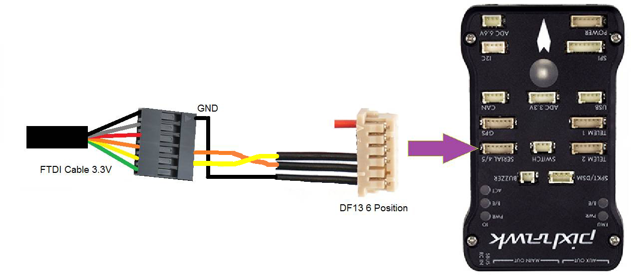

第二种方式为GCS：即通过飞控与地面站建立通信，在地面站上显示图形界面来显示波形。下面结合源码简单分析一下GCS：
从Arducopter.cpp可以看出，与地面站通信的主要线程为：

SCHED_TASK(gcs_check_input,      400,    180),
SCHED_TASK(gcs_send_heartbeat,     1,    110),
SCHED_TASK(gcs_send_deferred,     50,    550),
SCHED_TASK(gcs_data_stream_send,  50,    550),

但是有一个地方需要注意，在void Copter::init_ardupilot()函数中，有一个设置：

// Register the mavlink service callback. This will run
// anytime there are more than 5ms remaining in a call to
// hal.scheduler->delay.
hal.scheduler->register_delay_callback(mavlink_delay_cb_static, 5);

而这个函数为mavlink_delay_cb_static，追踪进去copter.mavlink_delay_cb();，再进去就是：

/*
 *  a delay() callback that processes MAVLink packets. We set this as the
 *  callback in long running library initialisation routines to allow
 *  MAVLink to process packets while waiting for the initialisation to
 *  complete
 */
void Copter::mavlink_delay_cb()
{
    static uint32_t last_1hz, last_50hz, last_5s;
    if (!gcs[0].initialised || in_mavlink_delay) return;

    in_mavlink_delay = true;

    uint32_t tnow = millis();
    if (tnow - last_1hz > 1000) {
        last_1hz = tnow;
        gcs_send_heartbeat();
        gcs_send_message(MSG_EXTENDED_STATUS1);
    }
    if (tnow - last_50hz > 20) {
        last_50hz = tnow;
        gcs_check_input();
        gcs_data_stream_send();
        gcs_send_deferred();
        notify.update();
    }
    if (tnow - last_5s > 5000) {
        last_5s = tnow;
        gcs_send_text(MAV_SEVERITY_INFO, "Initialising APM");
    }
    check_usb_mux();

    in_mavlink_delay = false;
}

可知在这里也进行了数据的发送，那岂不是与之前的线程冲突了？
仔细查看hal.scheduler->register_delay_callback这个函数:

void PX4Scheduler::register_delay_callback(AP_HAL::Proc proc,
                                            uint16_t min_time_ms) 
{
    _delay_cb = proc;
    _min_delay_cb_ms = min_time_ms;
}

而_delay_cb，_min_delay_cb_ms在delay函数里得到了调用：

void PX4Scheduler::delay(uint16_t ms)
{
    if (in_timerprocess()) {
        ::printf("ERROR: delay() from timer process\n");
        return;
    }
    perf_begin(_perf_delay);
	uint64_t start = AP_HAL::micros64();
    
    while ((AP_HAL::micros64() - start)/1000 < ms && 
           !_px4_thread_should_exit) {
        delay_microseconds_semaphore(1000);
        if (_min_delay_cb_ms <= ms) {
            if (_delay_cb) {
                _delay_cb();
            }
        }
    }
    perf_end(_perf_delay);
    if (_px4_thread_should_exit) {
        exit(1);
    }
}

因此可以知道这里的意思就是，如果系统有延时过长（_min_delay_cb_ms <= ms）的情况，则会给gcs发送数据，这样以防止与gcs通信中断。

主要发送消息流函数gcs_data_stream_send

/*
 *  send data streams in the given rate range on both links
 */
void Copter::gcs_data_stream_send(void)
{
    for (uint8_t i=0; i<num_gcs; i++) {
        if (gcs[i].initialised) {
            gcs[i].data_stream_send();
        }
    }
}

如果我们继续往里边看，可以看到这里分类进行输出。

void
GCS_MAVLINK::data_stream_send(void)
{
    if (waypoint_receiving) {
        // don't interfere with mission transfer
        return;
    }

    if (!copter.in_mavlink_delay && !copter.motors.armed()) {
        handle_log_send(copter.DataFlash);
    }

    copter.gcs_out_of_time = false;

    if (_queued_parameter != NULL) {
        if (streamRates[STREAM_PARAMS].get() <= 0) {
            streamRates[STREAM_PARAMS].set(10);
        }
        if (stream_trigger(STREAM_PARAMS)) {
            send_message(MSG_NEXT_PARAM);
        }
        // don't send anything else at the same time as parameters
        return;
    }

    if (copter.gcs_out_of_time) return;

    if (copter.in_mavlink_delay) {
        // don't send any other stream types while in the delay callback
        return;
    }

    if (stream_trigger(STREAM_RAW_SENSORS)) {
        send_message(MSG_RAW_IMU1);
        send_message(MSG_RAW_IMU2);
        send_message(MSG_RAW_IMU3);
    }

    if (copter.gcs_out_of_time) return;

    if (stream_trigger(STREAM_EXTENDED_STATUS)) {
        send_message(MSG_EXTENDED_STATUS1);
        send_message(MSG_EXTENDED_STATUS2);
        send_message(MSG_CURRENT_WAYPOINT);
        send_message(MSG_GPS_RAW);
        send_message(MSG_NAV_CONTROLLER_OUTPUT);
        send_message(MSG_LIMITS_STATUS);
    }

    if (copter.gcs_out_of_time) return;

    if (stream_trigger(STREAM_POSITION)) {
        send_message(MSG_LOCATION);
        send_message(MSG_LOCAL_POSITION);
    }

    if (copter.gcs_out_of_time) return;

    if (stream_trigger(STREAM_RAW_CONTROLLER)) {
        send_message(MSG_SERVO_OUT);
    }

    if (copter.gcs_out_of_time) return;

    if (stream_trigger(STREAM_RC_CHANNELS)) {
        send_message(MSG_RADIO_OUT);
        send_message(MSG_RADIO_IN);
    }

    if (copter.gcs_out_of_time) return;

    if (stream_trigger(STREAM_EXTRA1)) {
        send_message(MSG_ATTITUDE);
        send_message(MSG_SIMSTATE);
        send_message(MSG_PID_TUNING);
    }

    if (copter.gcs_out_of_time) return;

    if (stream_trigger(STREAM_EXTRA2)) {
        send_message(MSG_VFR_HUD);
    }

    if (copter.gcs_out_of_time) return;

    if (stream_trigger(STREAM_EXTRA3)) {
        send_message(MSG_AHRS);
        send_message(MSG_HWSTATUS);
        send_message(MSG_SYSTEM_TIME);
        send_message(MSG_RANGEFINDER);
#if AP_TERRAIN_AVAILABLE && AC_TERRAIN
        send_message(MSG_TERRAIN);
#endif
        send_message(MSG_BATTERY2);
        send_message(MSG_MOUNT_STATUS);
        send_message(MSG_OPTICAL_FLOW);
        send_message(MSG_GIMBAL_REPORT);
        send_message(MSG_MAG_CAL_REPORT);
        send_message(MSG_MAG_CAL_PROGRESS);
        send_message(MSG_EKF_STATUS_REPORT);
        send_message(MSG_VIBRATION);
        send_message(MSG_RPM);
    }
}

这么多消息，它的管理方式为队列。

// send a message using mavlink, handling message queueing
void GCS_MAVLINK::send_message(enum ap_message id)
{
    uint8_t i, nextid;

    // see if we can send the deferred messages, if any
    while (num_deferred_messages != 0) {
        if (!try_send_message(deferred_messages[next_deferred_message])) {
            break;
        }
        next_deferred_message++;
        if (next_deferred_message == MSG_RETRY_DEFERRED) {
            next_deferred_message = 0;
        }
        num_deferred_messages--;
    }

    if (id == MSG_RETRY_DEFERRED) {
        return;
    }

    // this message id might already be deferred
    for (i=0, nextid = next_deferred_message; i < num_deferred_messages; i++) {
        if (deferred_messages[nextid] == id) {
            // its already deferred, discard
            return;
        }
        nextid++;
        if (nextid == MSG_RETRY_DEFERRED) {
            nextid = 0;
        }
    }

    if (num_deferred_messages != 0 ||
        !try_send_message(id)) {
        // can't send it now, so defer it
        if (num_deferred_messages == MSG_RETRY_DEFERRED) {
            // the defer buffer is full, discard
            return;
        }
        nextid = next_deferred_message + num_deferred_messages;
        if (nextid >= MSG_RETRY_DEFERRED) {
            nextid -= MSG_RETRY_DEFERRED;
        }
        deferred_messages[nextid] = id;
        num_deferred_messages++;
    }
}

注意这里边有个所谓的get_secondary_attitude函数，它是另外一种算法的姿态信息，不是DCM就是EKF：

// return secondary attitude solution if available, as eulers in radians
bool AP_AHRS_NavEKF::get_secondary_attitude(Vector3f &eulers)
{
    switch (active_EKF_type()) {
    case EKF_TYPE_NONE:
        // EKF is secondary
        EKF1.getEulerAngles(eulers); //这个是EKF1算法生成的姿态信息
        return ekf1_started;

    case EKF_TYPE1:
    case EKF_TYPE2:
    default:
        // DCM is secondary
        eulers = _dcm_attitude; //这是DCM算法生成的姿态信息，应该是返回这里
        return true;
    }
}

消息由_mav_finalize_message_chan_send定制，最后由comm_send_buffer发出～
如果飞控出现问题如，gcs_send_text(MAV_SEVERITY_CRITICAL,”PreArm: Waiting for Nav Checks”);，是这个函数发出来的。

在apmplanner里查看波形如下：

第三种当然是通过SD卡咯，一般来说，当我们实际飞行完成后，可以将SD里面的飞行数据进行分析，对于APM的固件，数据打包成bin格式的文件存储于SD卡中，可以使用apmplanner(如上图中的OpenLog)读取，也可以通过MAVExplorer。实际操作很简单，不进行分析。
APM的源码体现为：

// fifty_hz_logging_loop
// should be run at 50hz
void Copter::fifty_hz_logging_loop()
{
#if HIL_MODE != HIL_MODE_DISABLED
    // HIL for a copter needs very fast update of the servo values
    gcs_send_message(MSG_RADIO_OUT);
#endif

#if HIL_MODE == HIL_MODE_DISABLED
    if (should_log(MASK_LOG_ATTITUDE_FAST)) {
        Log_Write_Attitude();
        Log_Write_Rate();
        if (should_log(MASK_LOG_PID)) {
            DataFlash.Log_Write_PID(LOG_PIDR_MSG, g.pid_rate_roll.get_pid_info() );
            DataFlash.Log_Write_PID(LOG_PIDP_MSG, g.pid_rate_pitch.get_pid_info() );
            DataFlash.Log_Write_PID(LOG_PIDY_MSG, g.pid_rate_yaw.get_pid_info() );
            DataFlash.Log_Write_PID(LOG_PIDA_MSG, g.pid_accel_z.get_pid_info() );
        }
    }

    // log IMU data if we're not already logging at the higher rate
    if (should_log(MASK_LOG_IMU) && !(should_log(MASK_LOG_IMU_FAST) || should_log(MASK_LOG_IMU_RAW))) {
        DataFlash.Log_Write_IMU(ins);
    }
#endif
}

参考文献

陀螺仪加速度计MPU6050

公众号:来风说

初学PX4之飞控算法